5.3 Parametric Methods - NOMINATE
5.3.3 Accessing DW-NOMINATE Scores
## Registered S3 methods overwritten by 'asmcjr':
##   method           from
##   end.mcmc.list    coda
##   start.mcmc.list  coda
##   window.mcmc      coda
##   window.mcmc.list coda
data(rcx)
# select the Congress terms of interest
ncong <- c(90, 100, 110)

# Filter the data for rows where the Congress number is in ncong and dist is not equal to 0
sub <- with(rcx, which(cong %in% ncong & dist != 0))

# Create a matrix containing the first dimension scores (dwnom1), party affiliation,
# and a factor indicating the Congress (e.g., "House 90", "House 100", "House 110")
polarization <- cbind(
  rcx[sub, c("dwnom1", "party")],  # Select columns for first dimension score and party
  congress = factor(paste("House", rcx$cong[sub]),  # Create a factor for the Congress
                    levels = c("House 90", "House 100", "House 110"))
)
library(ggplot2)

# Ensure that 'party' is a factor
polarization$party <- as.factor(polarization$party)

# Create the plot
ggplot(polarization, aes(x = dwnom1, group = party, colour = party, fill = party)) +
  geom_density(adjust = 2.5, alpha = .2) +
  facet_wrap(~congress, ncol = 2) +
  xlab("DW-Nominate\n(First Dimension)") +
  theme_bw() +
  scale_colour_manual(values = c("gray25", "gray75"), name = "Party") +
  scale_fill_manual(values = c("gray25", "gray75"), name = "Party") +
  theme(aspect.ratio = 1, legend.position = "bottom")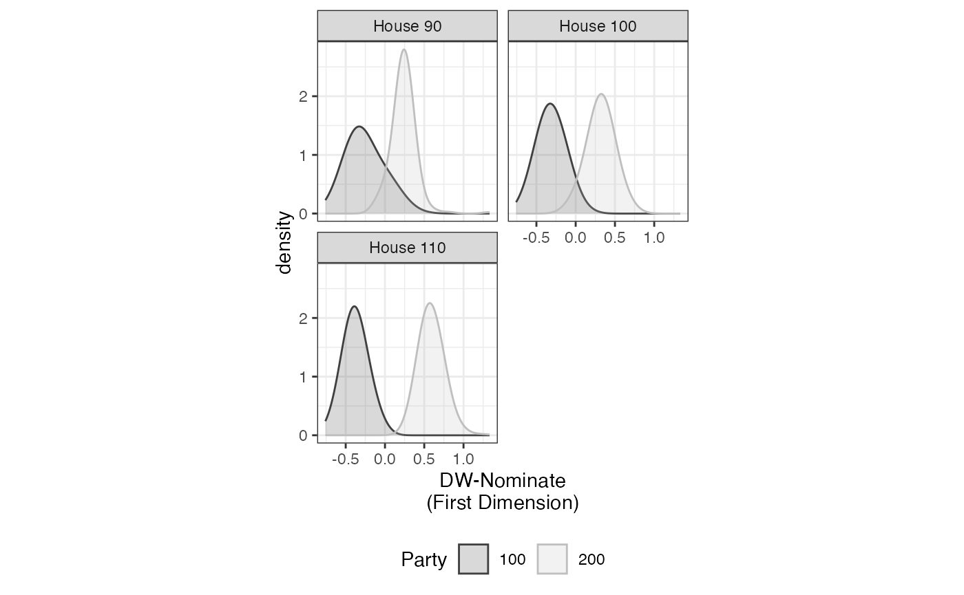
FIGURE 5.2: Partisan Polarization in the 90th, 100th, and 110th Houses
5.3.5 Example 1: The 108th US House
library(wnominate)
result <- wnominate(hr108, ubeta=15, uweights=0.5, dims=2,
                    minvotes=20, lop=0.025, trials=1, polarity=c(1,5), verbose=FALSE)
##
## Preparing to run W-NOMINATE...
##
## Checking data...
##
## All members meet minimum vote requirements.
##
## Votes dropped:
## ... 375 of 1218 total votes dropped.
##
## Running W-NOMINATE...
##
## Getting bill parameters...
## Getting legislator coordinates...
## Starting estimation of Beta...
## Getting bill parameters...
## Getting legislator coordinates...
## Starting estimation of Beta...
## Getting bill parameters...
## Getting legislator coordinates...
## Getting bill parameters...
## Getting legislator coordinates...
## Estimating weights...
## Getting bill parameters...
## Getting legislator coordinates...
## Estimating weights...
## Getting bill parameters...
## Getting legislator coordinates...
##
##
## W-NOMINATE estimation completed successfully.
## W-NOMINATE took 92.825 seconds to execute.Create a grouping variable based on partyCode and icpsrState.
group <- rep(NA, nrow(result$legislators))
group[with(result$legislators, which(partyCode == 100 & icpsrState %in% c(40:51, 53, 54)))] <- 1
group[with(result$legislators, which(partyCode == 100 & icpsrState %in% c(1:39, 52, 55:82)))] <- 2
group[with(result$legislators, which(partyCode == 200))] <- 3
group[with(result$legislators, which(partyCode == 328))] <- 4

# Convert the group variable to a factor with appropriate labels
group <- factor(group, levels = 1:4,
                labels = c("Southern Dems", "Northern Dems",
                           "Republicans", "Independents"))
library(ggplot2)
# Plot using plot_wnom_coords with customized colors and shapes
plot_wnom_coords(result, shapeVar = group, dropNV = FALSE) +
  scale_color_manual(values = gray.colors(4, end = .75), name = "Party Group",
                     labels = c("Southern Dems", "Northern Dems",
                                "Republicans", "Independents")) +
  scale_shape_manual(values = c("S", "N", "R", "I"), name = "Party Group",
                     labels = c("Southern Dems", "Northern Dems",
                                "Republicans", "Independents")) +
  theme_bw() +
  theme(aspect.ratio = 1, legend.position = "bottom") +
  xlab("First Dimension") +
  ylab("Second Dimension") +
  guides(colour = guide_legend(nrow = 2))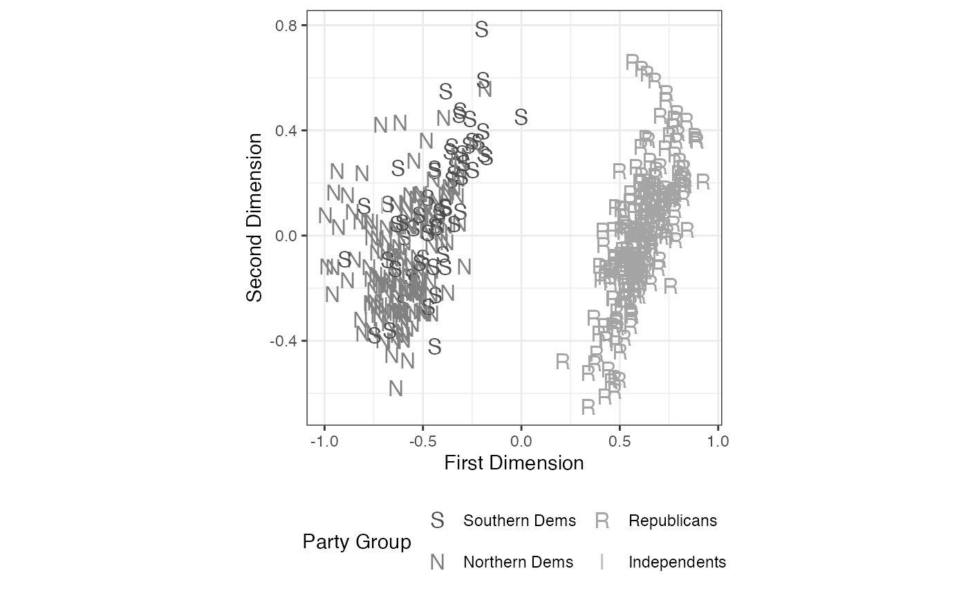
FIGURE 5.3: W-NOMINATE Ideal Point Estimates of Members of the 108th US House of Representatives
Shows the roll call choices of all voting legislators.
# Calculate the weight based on the result's weights
weight <-  result$weights[2] / result$weights[1]

# Create a data frame with the first and second dimension coordinates, adjusting the second dimension by the weight
wnom.dat <- data.frame(
  coord1D = result$legislators$coord1D,
  coord2D = result$legislators$coord2D * weight,
  group = group
)

# Plot the roll call results
plot_rollcall(result, hr108, wnom.dat, 528, wnom.dat$group, dropNV = TRUE) +
  theme_bw() +
  scale_shape_manual(values = c("S", "D", "R", "I"), name = "Party Group") +
  xlab("First Dimension") +
  ylab("Second Dimension") +
  theme(aspect.ratio = 1, legend.position = "bottom") +
  guides(shape = guide_legend(nrow = 2))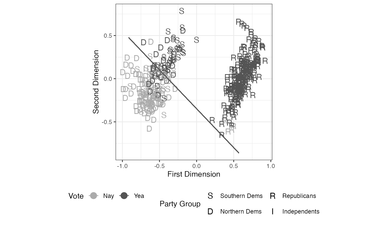
FIGURE 5.4: W-NOMINATE Analysis of the 108th House Vote on the Partial-Birth Abortion Ban Act of 2003, All Legislators
We can calculate the PRE (Proportional Reduction in Error) statistic and display it in the plot below the number of errors as below:
## $tot.errors
## yea_error nay_error
##        19        17
##
## $PRE
## [1] 0.7464789
To plot only those legislators who committed voting errors, we can use the plot_rollcall() function from above.
plot_rollcall(result, hr108, wnom.dat, 528,
             shapeVar=wnom.dat$group, onlyErrors=TRUE) +
  scale_shape_manual(values=c("S", "N", "R"), name="Party Group") +
  theme_bw() +
  theme(aspect.ratio=1, legend.position="bottom") +
  xlab("First Dimension") +
  ylab("Second Dimension") +
  guides(shape = guide_legend(nrow=2))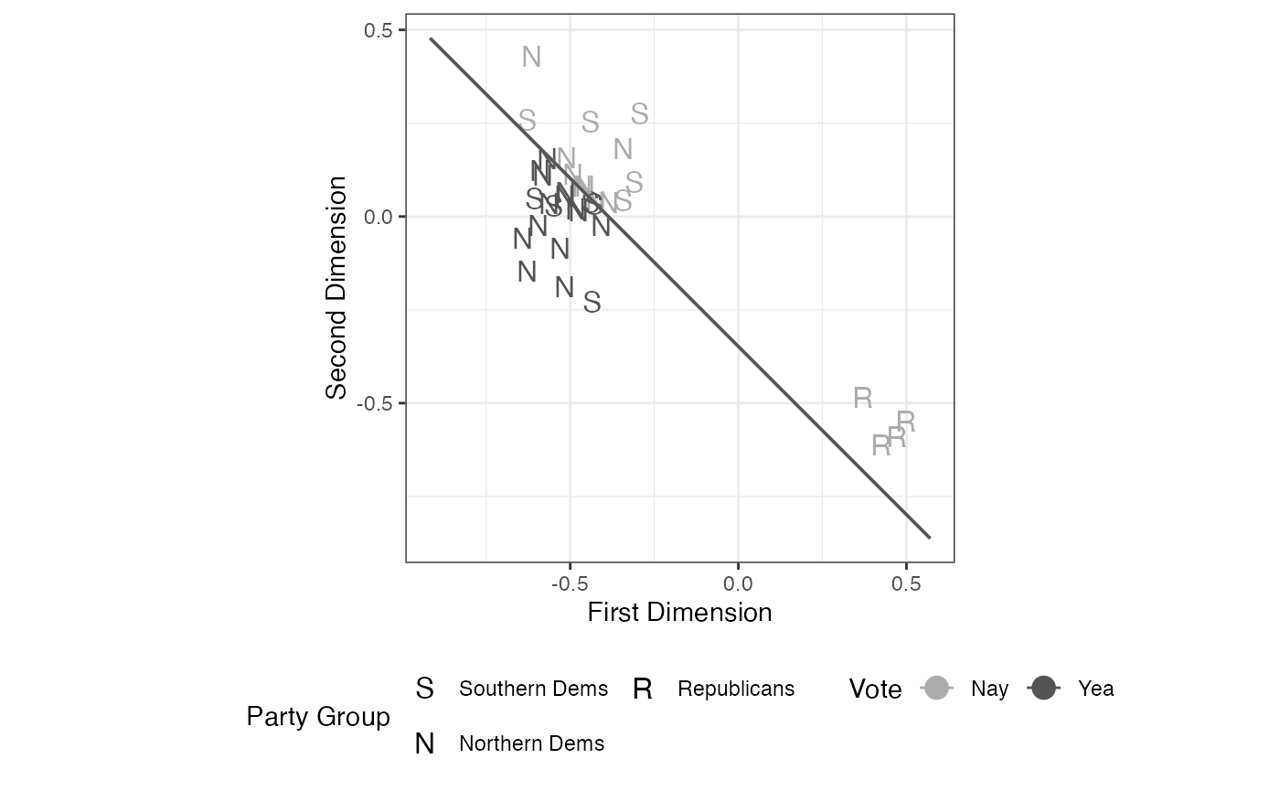
FIGURE 5.5: W-NOMINATE Analysis of the 108th House Vote on the Partial-Birth Abortion Ban Act of 2003, Errors Only
5.3.5.3 The Coombs Mesh and Cutting Line Angles
The Coombs mesh also illustrates how cutting planes intersect to form polytopes (bounded regions in the space).
angles <- makeCutlineAngles(result)
head(angles)
## angle N1W N2W
## 1 69.71863 0.9380017 -0.34663060
## 2 69.61088 0.9373482 -0.34839406
## 3 70.86382 0.9447421 -0.32781452
## 4 70.74404 0.9440547 -0.32978881
## 5 87.50801 0.9990543 -0.04347964
## 6 NA NA NA
print(angles[528,])## angle N1W N2W
## 528 -42.01419 0.6693147 0.742979## [1] 68.5467
ggplot(angles, aes(x=angle)) +
     geom_histogram() +
     theme_bw() +
     theme(aspect.ratio=1) +
     xlab("Cutline Angles")
## `stat_bin()` using `bins = 30`. Pick better value with `binwidth`.## Warning: Removed 375 rows containing non-finite outside the scale range
## (`stat_bin()`).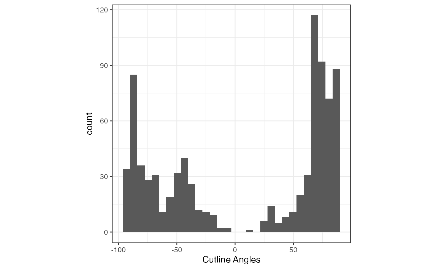
FIGURE 5.7: Histogram of Cutting Line Angles of Roll Call Votes in the 108th US House
5.3.6 Example 2: The First European Parliament (Using the Parametric Bootstrap)
library(wnominate)
result <- wnominate(rc_ep, ubeta=15, uweights=0.5, dims=2, minvotes=20,
                    lop=0.025, trials=5, polarity=c(25,25), verbose=FALSE)
##
## Preparing to run W-NOMINATE...
##
## Checking data...
##
## ... 38 of 548 total members dropped.
##
## Votes dropped:
## ... 97 of 886 total votes dropped.
##
## Running W-NOMINATE...
##
## Getting bill parameters...
## Getting legislator coordinates...
## Starting estimation of Beta...
## Getting bill parameters...
## Getting legislator coordinates...
## Starting estimation of Beta...
## Getting bill parameters...
## Getting legislator coordinates...
## Getting bill parameters...
## Getting legislator coordinates...
## Estimating weights...
## Getting bill parameters...
## Getting legislator coordinates...
## Estimating weights...
## Getting bill parameters...
## Getting legislator coordinates...
## Starting bootstrap iterations...
## ... Computing standard errors...
## W-NOMINATE estimation completed successfully.
## W-NOMINATE took 1138.505 seconds to execute.
library(ggplot2)
plot_wnom_coords(result, shapeVar = result$legislators$MS,
                 dropNV = FALSE, ptSize = 4, ci = FALSE) +
  scale_shape_discrete(name = "Party Group")
## Warning: The shape palette can deal with a maximum of 6 discrete values because more
## than 6 becomes difficult to discriminate
## ℹ you have requested 11 values. Consider specifying shapes manually if you need
## that many have them.## Warning: Removed 191 rows containing missing values or values outside the scale range
## (`geom_point()`).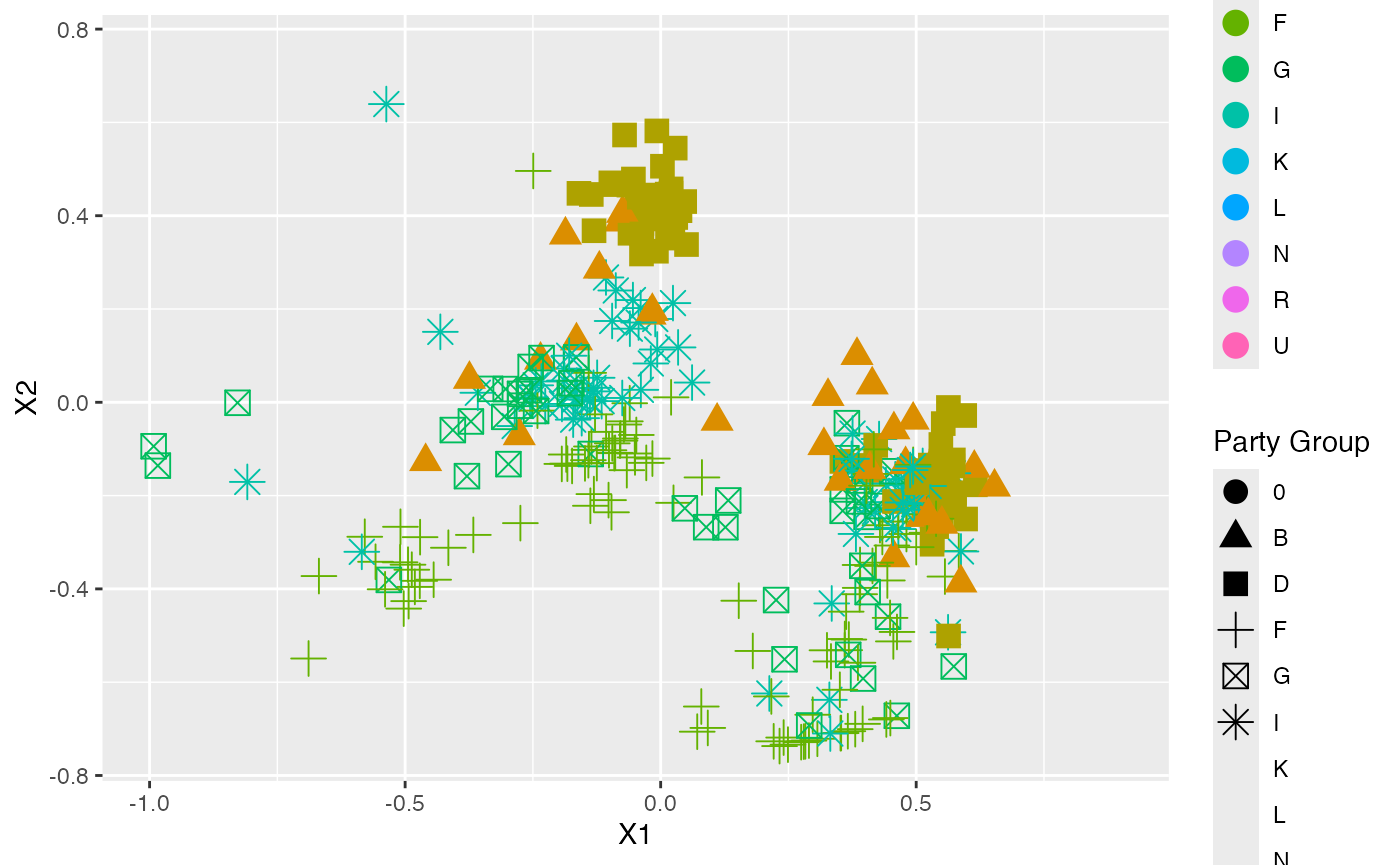
FIGURE 5.8: W-NOMINATE Ideal Point Estimates of Members of the First European Parliament
5.4 Nonparametric Methods - Optimal Classification
5.4.2 Example 1: The French National Assembly during the Fourth Republic
library(asmcjr)
data(france4)
rc <- rollcall(data=france4[,6:ncol(france4)],
   yea=1,
   nay=6,
   missing=7,
   notInLegis=c(8,9),
   legis.names=paste(france4$NAME,france4$CASEID,sep=""),
   vote.names=colnames(france4[6:ncol(france4)]),
   legis.data=france4[,2:5],
   vote.data=NULL,
desc="National Assembly of the French Fourth Republic")##
## Preparing to run Optimal Classification...
##
## Checking data...
##
## ... 112 of 1566 total members dropped.
##
## Votes dropped:
## ... 34 of 889 total votes dropped.
##
## Running Optimal Classification...
##
## Generating Start Coordinates...
## Running Edith Algorithm...
## Permuting adjacent legislator pairs...
## Permuting adjacent legislator triples...
##
##
## Optimal Classification completed successfully.
## Optimal Classification took 934.042 seconds to execute.##
## Preparing to run Optimal Classification...
##
## Checking data...
##
## ... 112 of 1566 total members dropped.
##
## Votes dropped:
## ... 34 of 889 total votes dropped.
##
## Running Optimal Classification...
##
## Generating Start Coordinates...
## Running Edith Algorithm...
## Getting normal vectors...
## Getting legislator coordinates...
## Getting normal vectors...
## Getting legislator coordinates...
## Getting normal vectors...
## Getting legislator coordinates...
## Getting normal vectors...
## Getting legislator coordinates...
## Getting normal vectors...
## Getting legislator coordinates...
## Getting normal vectors...
## Getting legislator coordinates...
## Getting normal vectors...
## Getting legislator coordinates...
## Getting normal vectors...
## Getting legislator coordinates...
## Getting normal vectors...
## Getting legislator coordinates...
## Getting normal vectors...
## Getting legislator coordinates...
##
##
## Optimal Classification completed successfully.
## Optimal Classification took 235.42 seconds to execute.