4.2 Metric Unfolding Using the MLSMU6 Procedure
4.2.1 Example 1: 1981 Interest Group Ratings of US Senators Data
## Registered S3 methods overwritten by 'asmcjr':
##   method           from
##   end.mcmc.list    coda
##   start.mcmc.list  coda
##   window.mcmc      coda
## window.mcmc.list codaThe data interest1981 are arranged such that the individuals (Senators) are on the rows and the stimuli (the interest groups) are on the columns. The interest group ratings themselves are stored in columns 9-38, which we assign to the matrix input.
# Convert selected columns (9 to 38) from the dataframe to a matrix
input <- as.matrix(interest1981[, 9:38])

# Set a cutoff threshold for the number of non-missing values required per row
cutoff <- 5

# Filter the rows to keep only those with at least 'cutoff' non-missing values
input <- input[rowSums(!is.na(input)) >= cutoff, ]

# Normalize the data by subtracting from 100 and dividing by 50
input <- (100 - input) / 50

# Square the normalized data
input2 <- input * input

# Replace NA values in the squared data with the square of the mean of non-NA values
input2[is.na(input)] <- (mean(input, na.rm = TRUE))^2
use double-centering to get good starting values for the MLSMU6 algorithm.
inputDC <- doubleCenterRect(input2)In order to obtain the starting coordinates for the stimuli (stims) and individuals (inds), we perform singular value decomposition on the double-centered matrix using the base function svd.
# Perform Singular Value Decomposition (SVD) on the input matrix
xsvd <- svd(inputDC)

# Set the number of dimensions to retain
ndim <- 2

# Extract the first 'ndim' right singular vectors (stimuli) and left singular vectors (individuals)
stims <- xsvd$v[, 1:ndim]
inds <- xsvd$u[, 1:ndim]

# Adjust the singular vectors by multiplying by the square root of the corresponding singular values
for (i in 1:ndim) {
  stims[,i] <- stims[,i] * sqrt(xsvd$d[i])
  inds[,i] <- inds[,i] * sqrt(xsvd$d[i])
}
MLSMU6 converges on the result for the 1981 interest
group data in 12 iterations, reducing the sum of squared errors to
194.132 (this information is stored in the iter element of the returned
results from the mlsmu6 procedure).
out <- mlsmu6(input = interest1981[,9:38], ndim=2, cutoff=5,
              id=factor(interest1981$party, labels=c("D", "R")))
tail(out$iter)
## iter ErrorSS
## [7,] 7 195.5551
## [8,] 8 194.9194
## [9,] 9 194.5672
## [10,] 10 194.3567
## [11,] 11 194.2225
## [12,] 12 194.1323
plot(out)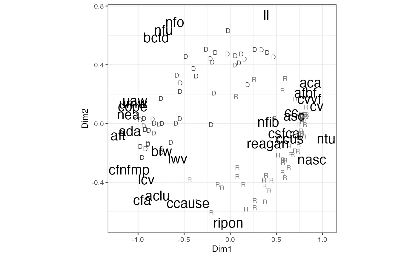
FIGURE 4.1: Metric Unfolding of 1981 Interest Group Ratings Data Using the MLSMU6 Procedure
| Code | Interest Group Name |
|---|---|
| ACLU | American Civil Liberties Union |
| ADA | Americans for Democratic Action |
| AFT | American Federation of Teachers |
| CC | Conservative Coalition (CQ) |
| CCAUSE | Common Cause |
| CCUS | Chamber of Commerce of the United States |
| COPE | Committee on Political Education AFL-CIO |
| LL | Liberty Lobby |
| NFIB | National Federation of Independent Business |
| NFU | National Farmers Union |
| NTU | National Taxpayers’ Union |
| RIPON | Ripon Society |
4.3 Metric Unfolding Using Majorization (SMACOF)
4.3.1 Example 1: 2009 European Election Study (Danish Module)
# Load the smacof package
library(smacof)
## Loading required package: plotrix## Loading required package: colorspace## Loading required package: e1071##
## Attaching package: 'smacof'## The following object is masked from 'package:base':
##
## transform
# Load the denmarkEES2009 dataset
data(denmarkEES2009)

# Extract columns related to voting propensity and convert them to a matrix
input.den <- as.matrix(denmarkEES2009[,c("q39_p1","q39_p2","q39_p3",
                                         "q39_p4","q39_p5","q39_p6","q39_p7","q39_p8")])

# Assign names to the columns, representing different political parties
colnames(input.den) <- c("Social Democrats",
                         "Danish Social Liberal Party", "Conservative Peoples Party",
                         "Socialist Peoples Party", "Danish Peoples Party",
                         "Liberal Party", "Liberal Alliance", "June Movement")

# Treat specific values (77, 88, 89) as missing values and replace them with NA
input.den[input.den == 77 | input.den == 88 | input.den == 89] <- NA

# Transform the voting propensity ratings into distances. The ratings are on a 0-10 scale,
# so they are subtracted from 10 and divided by 5, resulting in distances ranging from 0 to 2.
input.den <- (10 - input.den) / 5

# Set a cutoff value to filter respondents who provided at least 5 party ratings
cutoff <- 5
input.den <- input.den[rowSums(!is.na(input.den)) >= cutoff,]
# Create the weight matrix with the same dimensions as input.den
weightmat <- input.den

# Assign 1 to cells with non-missing values in input.den
weightmat[!is.na(input.den)] <- 1

# Assign 0 to cells with missing values in input.den
weightmat[is.na(input.den)] <- 0

# Replace missing values in input.den with the mean of the non-missing values
input.den[is.na(input.den)] <- mean(input.den, na.rm = TRUE)
library(smacof)
result <- smacofRect(delta=input.den, ndim=2, itmax=1000,
                     weightmat=weightmat, init=NULL, verbose=FALSE)
# Extract estimated coordinates of voters and parties
voters <- result$conf.row
parties <- result$conf.col

# Check if the first dimension score for the first party is positive
if (parties[1,1] > 0) {
  # If positive, flip the signs of the first dimension for both parties and voters
  parties[,1] <- -1 * parties[,1]
  voters[,1] <- -1 * voters[,1]
}
# Create data frame for voters
voters.dat <- data.frame(
   dim1 = voters[,1],
   dim2 = voters[,2]
)

# Create data frame for parties
parties.dat <- data.frame(
   dim1 = parties[,1],
   dim2 = parties[,2],
   party = factor(1:8, labels=rownames(parties))
)
library(ggplot2)
g <- ggplot() +
   geom_point(data = voters.dat, aes(x=dim1, y=dim2), pch=1, color="gray65") +
   geom_point(data=parties.dat, aes(x=dim1, y=dim2), size=2.5) +
   geom_text(data=parties.dat, aes(x=dim1, y=dim2, label = party), nudge_y=.1, size=5) +
   theme_bw() +
   labs(x="First Dimension", y="Second Dimension") +
   theme(aspect.ratio=1)

g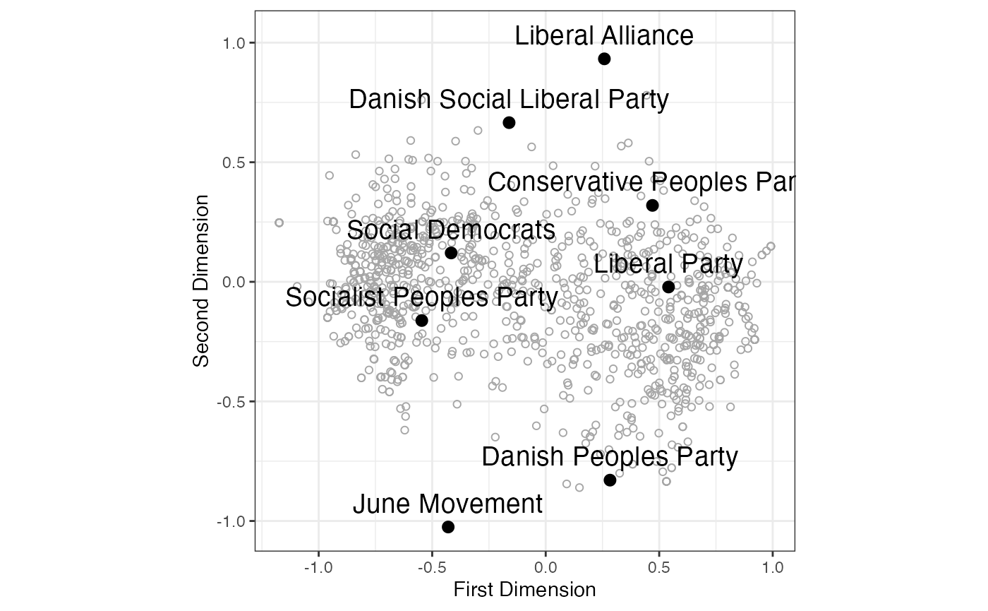
FIGURE 4.2: SMACOF (Majorization) Metric Unfolding of Propensity to Vote Ratings of Danish Political Parties (2009 European Election Study)
To understand the relationship between the Aldrich-McKelvey (AM) estimates of the parties’ left-right positions and their scores on the first and second dimensions obtained from a spatial analysis.
# Perform OLS regression to model the relationship between the Aldrich-McKelvey
library(basicspace)
AM.result <- aldmck(input.den,polarity=2,
     missing=c(77,88,89), verbose=FALSE)
# estimates of the parties' left-right positions and their scores on the first and second dimensions
ols <- lm(AM.result$stimuli ~ parties[,1] + parties[,2])

# Print the coefficients, standard errors, t-values, and p-values from the regression model
printCoefmat(summary(ols)$coefficients)
## Estimate Std. Error t value Pr(>|t|)
## (Intercept) 3.3217e-14 5.3634e-02 0.0000 1.000000
## parties[, 1] 8.3248e-01 1.3516e-01 6.1594 0.001641 **
## parties[, 2] -1.9535e-01 8.7642e-02 -2.2289 0.076268 .
## ---
## Signif. codes: 0 '***' 0.001 '**' 0.01 '*' 0.05 '.' 0.1 ' ' 1
# Calculate N1 and N2 from the regression coefficients
N1 <- ols$coefficients[2] /
      sqrt((ols$coefficients[2]^2) + (ols$coefficients[3]^2))

N2 <- ols$coefficients[3] /
      sqrt((ols$coefficients[2]^2) + (ols$coefficients[3]^2))

# Print the results
cat("N1 =", N1, "\n")
## N1 = 0.9735552
cat("N2 =", N2, "\n")## N2 = -0.2284518
# Normal vector (N1, N2) segment
exp.factor <- 1.1
g <- g + geom_segment(aes(x=exp.factor*-N1, y=exp.factor*-N2,
                          xend=exp.factor*N1, yend=exp.factor*N2),
                      lty=2, linewidth=1)

# Display the plot
print(g)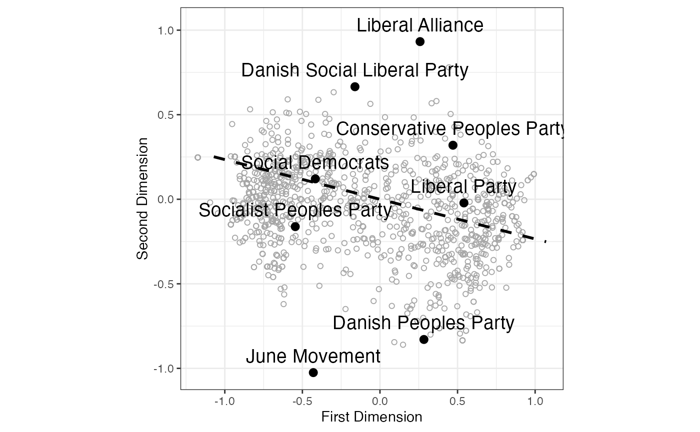
FIGURE 4.3: SMACOF (Majorization) Metric Unfolding of Propensity to Vote Ratings of Danish Political Parties (2009 Eu- ropean Election Study) with Normal Vector of Left-Right Scores