2.1.2 Example 1: 2009 European Election Study (French Module)
## Registered S3 methods overwritten by 'asmcjr':
##   method           from
##   end.mcmc.list    coda
##   start.mcmc.list  coda
##   window.mcmc      coda
## window.mcmc.list coda## self Extreme Left Communist Socialist Greens UDF (Bayrou) UMP (Sarkozy)
## [1,] 77 0 0 1 5 5 9
## [2,] 77 0 5 4 5 89 8
## [3,] 77 89 89 89 89 6 89
## [4,] 3 89 89 89 89 89 89
## [5,] 77 77 77 77 77 77 77
## [6,] 5 0 0 3 89 0 89
## National Front Left Party
## [1,] 10 1
## [2,] 10 4
## [3,] 10 89
## [4,] 89 89
## [5,] 77 77
## [6,] 89 5
library(basicspace)## Loading required package: tools##
## ## BASIC SPACE SCALING PACKAGE## ## 2009 - 2024## ## Keith Poole, Howard Rosenthal, Jeffrey Lewis, James Lo, and Royce Carroll## ## Support provided by the U.S. National Science Foundation## ## NSF Grant SES-0611974
result.france <- aldmck(franceEES2009, respondent=1, polarity=2,
     missing=c(77,88,89), verbose=FALSE)
# plot stimuli locations in addition to ideal point density
library(ggplot2)
# plot density of ideal points
plot_resphist(result.france, xlab="Left-Right")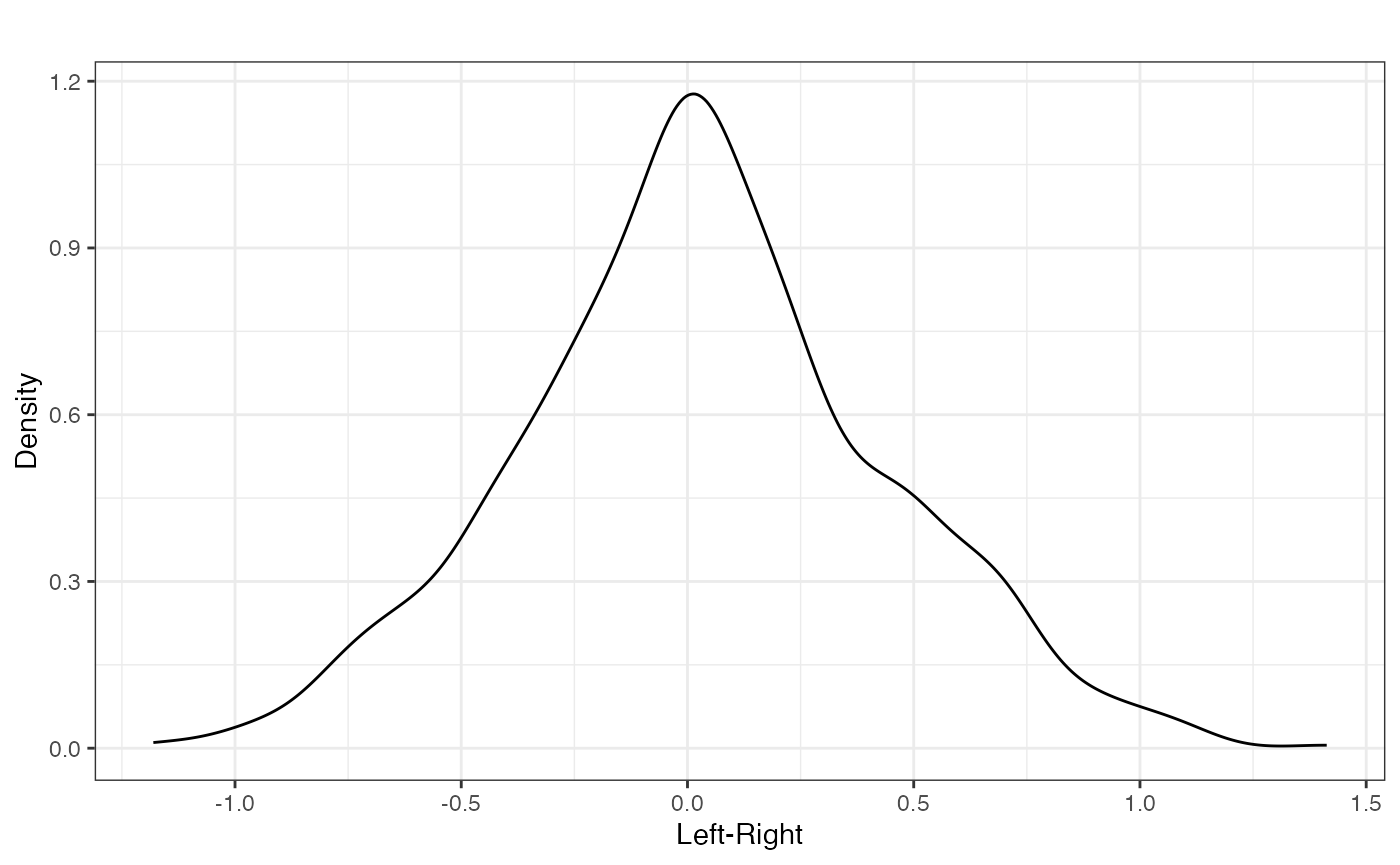
FIGURE 2.1: Aldrich-McKelvey Scaling of Left-Right Self- Placements of French Respondents (2009 European Election Study)
# plot stimuli locations in addition to ideal point density
plot_resphist(result.france, addStim=TRUE, xlab = "Left-Right") +
  theme(legend.position="bottom", aspect.ratio=1) +
  guides(shape = guide_legend(override.aes = list(size = 4), nrow=3)) +
 labs(shape="Party", colour="Party")
## Warning: The `guide` argument in `scale_*()` cannot be `FALSE`. This was deprecated in
## ggplot2 3.3.4.
## ℹ Please use "none" instead.
## ℹ The deprecated feature was likely used in the asmcjr package.
## Please report the issue at <https://github.com/uniofessex/asmcjr/issues>.
## This warning is displayed once every 8 hours.
## Call `lifecycle::last_lifecycle_warnings()` to see where this warning was
## generated.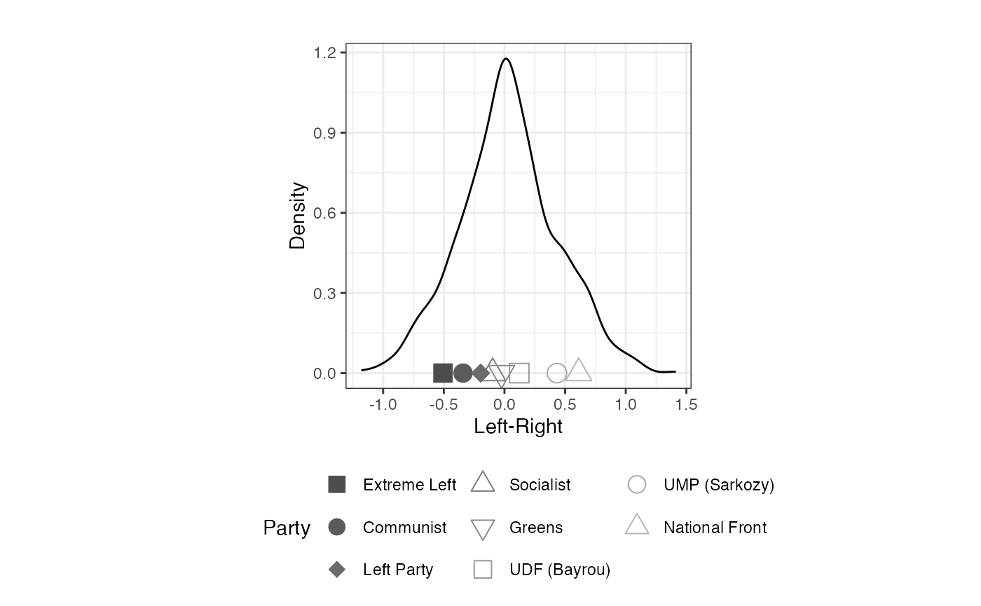
FIGURE 2.2: Aldrich-McKelvey Scaling of Left-Right Placements of French Political Parties (2009 European Election Study)
# isolate positive weights
plot_resphist(result.france, addStim=TRUE, weights="positive",
              xlab = "Left-Right")  +
  theme(legend.position="bottom", aspect.ratio=1) +
  guides(shape = guide_legend(override.aes = list(size = 4), nrow=3)) +
  labs(shape="Party", colour="Party")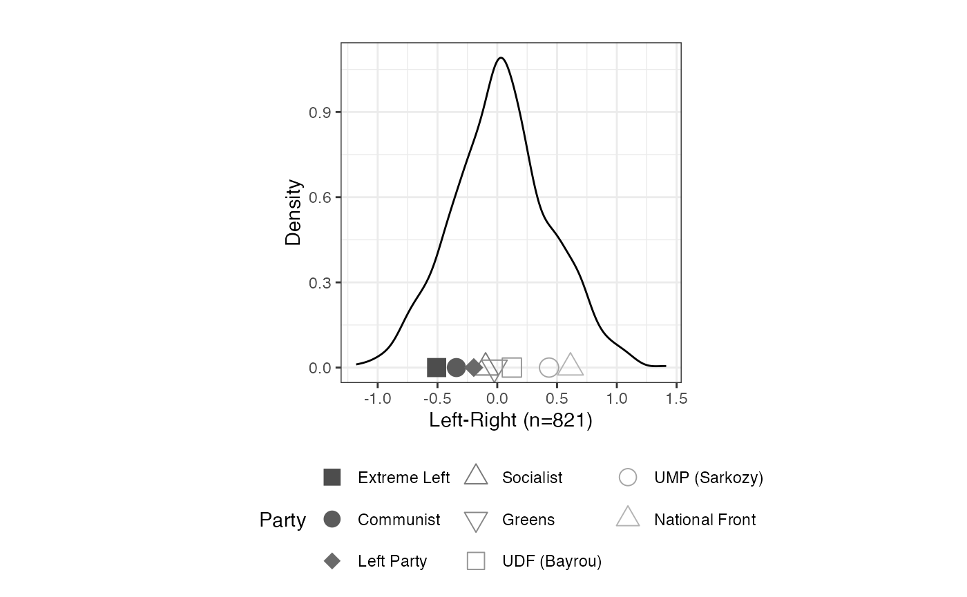
FIGURE 2.3: Aldrich-McKelvey Scaling of Left-Right Placements of French Political Parties: Positive Weights (2009 European Election Study)
# isolate positive weights
plot_resphist(result.france, addStim=TRUE,
              weights="negative", xlab = "Left-Right")  +
  theme(legend.position="bottom", aspect.ratio=1) +
  guides(shape = guide_legend(override.aes = list(size = 4), nrow=3)) +
  labs(shape="Party", colour="Party")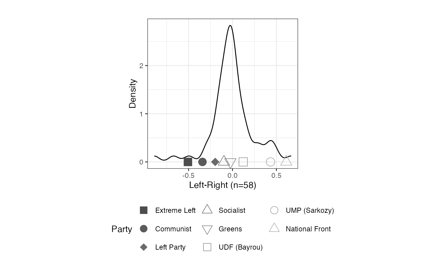
FIGURE 2.3: Aldrich-McKelvey Scaling of Left-Right Placements of French Political Parties: Negative Weights (2009 European Election Study)
2.1.3 Example 2: 1968 American National Election Study Urban Unrest and Vietnam War Scales
Urban Unrest
Running Bayesian Aldrich-Mckelvey
# Loading 'nes1968_urbanunrest'
data(nes1968_urbanunrest)
# Creating object with US president left-right dimensions
urban <- as.matrix(nes1968_urbanunrest[,-1])
# Running Bayesian Aldrich-Mckelvey scaling on President positions
library(basicspace)
result.urb <- aldmck(urban, polarity=2, respondent=5,
                     missing=c(8,9), verbose=FALSE)
summary(result.urb)
##
##
## SUMMARY OF ALDRICH-MCKELVEY OBJECT
## ----------------------------------
##
## Number of Stimuli: 4
## Number of Respondents Scaled: 1191
## Number of Respondents (Positive Weights): 1110
## Number of Respondents (Negative Weights): 81
## Reduction of normalized variance of perceptions: 0.09
##
## Location
## Humphrey -0.428
## Johnson -0.399
## Nixon 0.015
## Wallace 0.811Extracting vote.choice Column
# recode so that only Humphrey, Nixon and Wallace are present
vote <- car:::recode(nes1968_urbanunrest[,1], "3='Humphrey'; 5 = 'Nixon'; 6 = 'Wallace'; else=NA",
                     as.factor=FALSE)
# Convert vote to factor with appropriate levels
vote <- factor(vote, levels=c("Humphrey", "Nixon", "Wallace"))
# Plot population distribution by vote choice
plot_resphist(result.urb, groupVar=vote, addStim=TRUE,
              xlab="Liberal-Conservative")  +
  theme(legend.position="bottom", aspect.ratio=1)  +
  guides(shape = guide_legend(override.aes =
                                list(size = 4, color=c("gray25", "gray50", "gray75"))),
  colour = "none") +
  xlim(c(-2,2)) +
  labs(shape="Candidate")
## Warning: Removed 451 rows containing missing values or values outside the scale range
## (`geom_line()`).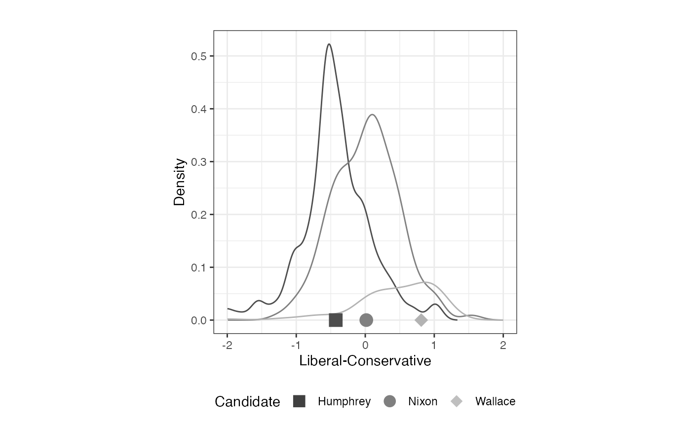
FIGURE 2.5: Aldrich-McKelvey Scaling of Urban Unrest Scale: Candidates and Voters (1968 American National Election Study)
Vietnam War Scales
data(nes1968_vietnam)
vietnam <- as.matrix(nes1968_vietnam[,-1])
# Aldrich-Mckelvey function for vietnam dataset
result.viet <- aldmck(vietnam, polarity=2, respondent=5,
                      missing=c(8,9), verbose=FALSE)
summary(result.viet)
##
##
## SUMMARY OF ALDRICH-MCKELVEY OBJECT
## ----------------------------------
##
## Number of Stimuli: 4
## Number of Respondents Scaled: 1031
## Number of Respondents (Positive Weights): 800
## Number of Respondents (Negative Weights): 231
## Reduction of normalized variance of perceptions: 0.19
##
## Location
## Humphrey -0.436
## Johnson -0.330
## Nixon -0.068
## Wallace 0.834
# Plot population distribution by vote choice
plot_resphist(result.urb, groupVar=vote, addStim=TRUE,
              xlab="Liberal-Conservative")  +
  theme(legend.position="bottom", aspect.ratio=1)  +
  guides(shape = guide_legend(override.aes =
                                list(size = 4, color=c("gray25", "gray50", "gray75"))),
  colour = "none") +
  xlim(c(-2,2)) +
  labs(shape="Candidate")
## Warning: Removed 451 rows containing missing values or values outside the scale range
## (`geom_line()`).
FIGURE 2.6: Aldrich-McKelvey Scaling of Vietnam War Scale: Candidates and Voters (1968 American National Election Study)
boot.france  <- boot.aldmck(franceEES2009,
                            polarity=2, respondent=1, missing=c(77,88,89),
                            verbose=FALSE, boot.args = list(R=100))
library(ggplot2)
ggplot(boot.france$sumstats, aes(x = idealpt, y = stimulus)) +
  geom_point() +
  # geom_errorbarh(aes(xmin = lower, xmax = upper), height = 0.2) +
  xlab("Left-Right") +
  ylab(NULL) +
  theme_minimal() +
theme(legend.position = "bottom", aspect.ratio = 1) 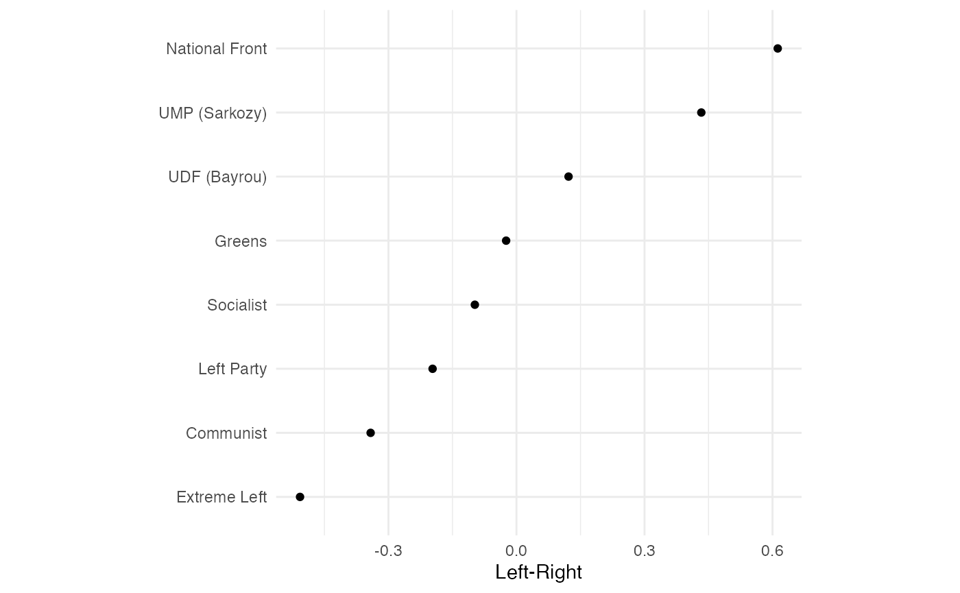
FIGURE 2.7: Aldrich-McKelvey Scaling of Left-Right Placements of French Political Parties (2009 European Election Study) with Bootstrapped Standard Errors
2.2.1 Example 1: 2000 Convention Delegate Study
##      Lib-Con Abortion Govt Services Defense Spending
## [1,]       3        4             5                4
## [2,]       2        4             5                6
## [3,]       1        4             7                6
## [4,]       2       99             6                5
## [5,]       4        4             7                1
## [6,]       4        4             7                4
Blackbox syntax of Republican-Democrat left-right scale
issues <- as.matrix(CDS2000[,5:14])
result.repdem <- blackbox(issues,
                          missing=99, dims=3, minscale=5, verbose=TRUE)
##
##
## Beginning Blackbox Scaling...10 stimuli have been provided.
##
## Blackbox estimation completed successfully.Recode party: Democrats = 1; Republicans = 2
party <- car:::recode(CDS2000[,1],
                      "1='Democrat'; 2='Republican'; else=NA",
                      as.factor=TRUE)
plot_blackbox(result.repdem, dims=c(1,2), groupVar=party,
              xlab= "First Dimension\n(Left-Right)",
              ylab="Second Dimension") +
  theme(legend.position="bottom", aspect.ratio=1) +
  guides(shape=guide_legend(override.aes=list(size=4))) +
  labs(colour="Party")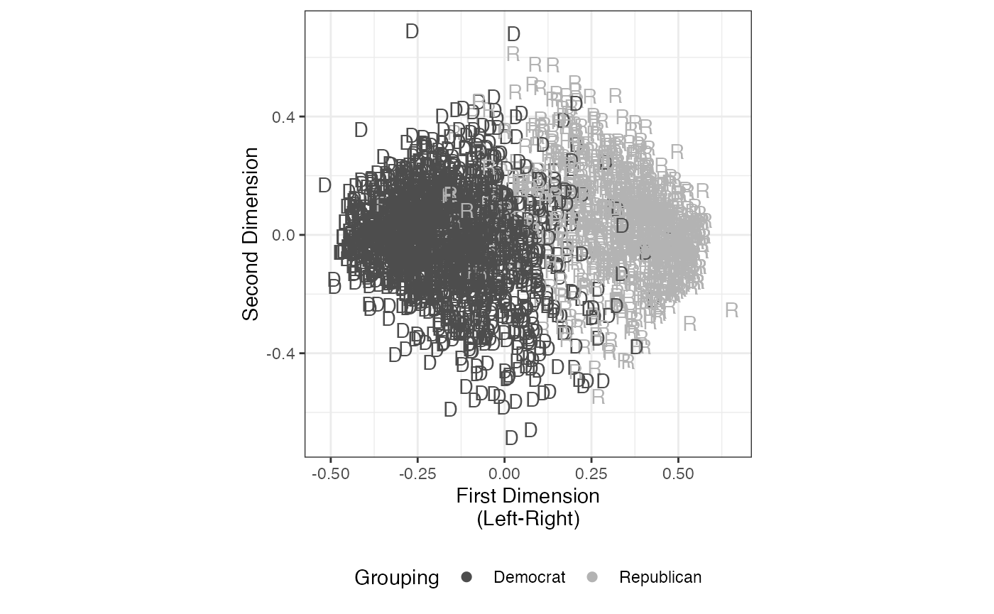
FIGURE 2.8: Basic Space (Blackbox) Scaling of US Party Conven- tion Delegates (2000 Convention Delegate Study)
2.2.2 Example 2: 2010 Swedish Parliamentary Candidate Survey
##      id elected         party.name party.code govt.party left.right.self.fivept
## 1 39681       0 Conservative Party        300          1                      5
## 2 17735       1 Conservative Party        300          1                      5
## 3 41923       0 Conservative Party        300          1                      4
## 4 43665       0 Conservative Party        300          1                      5
## 5 15867       0 Conservative Party        300          1                      5
## 6 39829       0 Conservative Party        300          1                      4
##   congestion.taxes highspeed.trains
## 1                3                2
## 2                3                3
## 3                4                1
## 4                4                2
## 5                3                3
## 6                2                2
Blacbox Scaling for Sweden issue scale
# Extract issues scales and convert to numeric
issues.sweden <- as.matrix(Sweden2010[,7:56])
mode(issues.sweden) <- "numeric"
# Blacbox syntax for Sweden issue scale
result.sweden <- blackbox(issues.sweden, missing=8,
                          dims=3, minscale=5, verbose=FALSE)
 # change polarity of scores
 if(result.sweden$individuals[[1]][13,1] < 0)
 result.sweden$individuals[[1]][,1] <-
     result.sweden$individuals[[1]][,1] * -1
 result.sweden$fits
## SSE SSE.explained percent SE singular
## Dimension 1 81259.51 91466.73 52.954739 0.8069252 255.24828
## Dimension 2 73388.39 99337.86 4.556993 0.7755642 92.78285
## Dimension 3 67238.03 105488.22 3.560756 0.7509879 85.00461
result.sweden$stimuli[[1]][16:25,]## N c w1 R2
## property.taxes.wealthy 2594 2.271 3.615 0.787
## wealth.tax 2621 1.983 3.420 0.793
## tax.wealthy 2652 2.337 3.635 0.820
## tax.pensions 2561 3.013 1.951 0.364
## household.services.deduction 2663 2.956 -3.726 0.809
## work.income.tax 2617 2.992 -2.553 0.588
## sex.purchase 2544 1.454 -0.736 0.084
## DUI.penalty 2537 3.384 -0.437 0.033
## criminal.sentences 2497 3.103 -1.461 0.278
## wiretaps 2393 2.786 2.732 0.553
elected <- as.numeric(Sweden2010[,2])
party.name.sweden <- as.factor(Sweden2010[,3])
plot_resphist(result.sweden, groupVar=party.name.sweden, dim=1,
              scaleDensity=FALSE) +
   facet_wrap(~stimulus, ncol=2) +
   theme(legend.position="none") +
   scale_color_manual(values=rep("black", 10))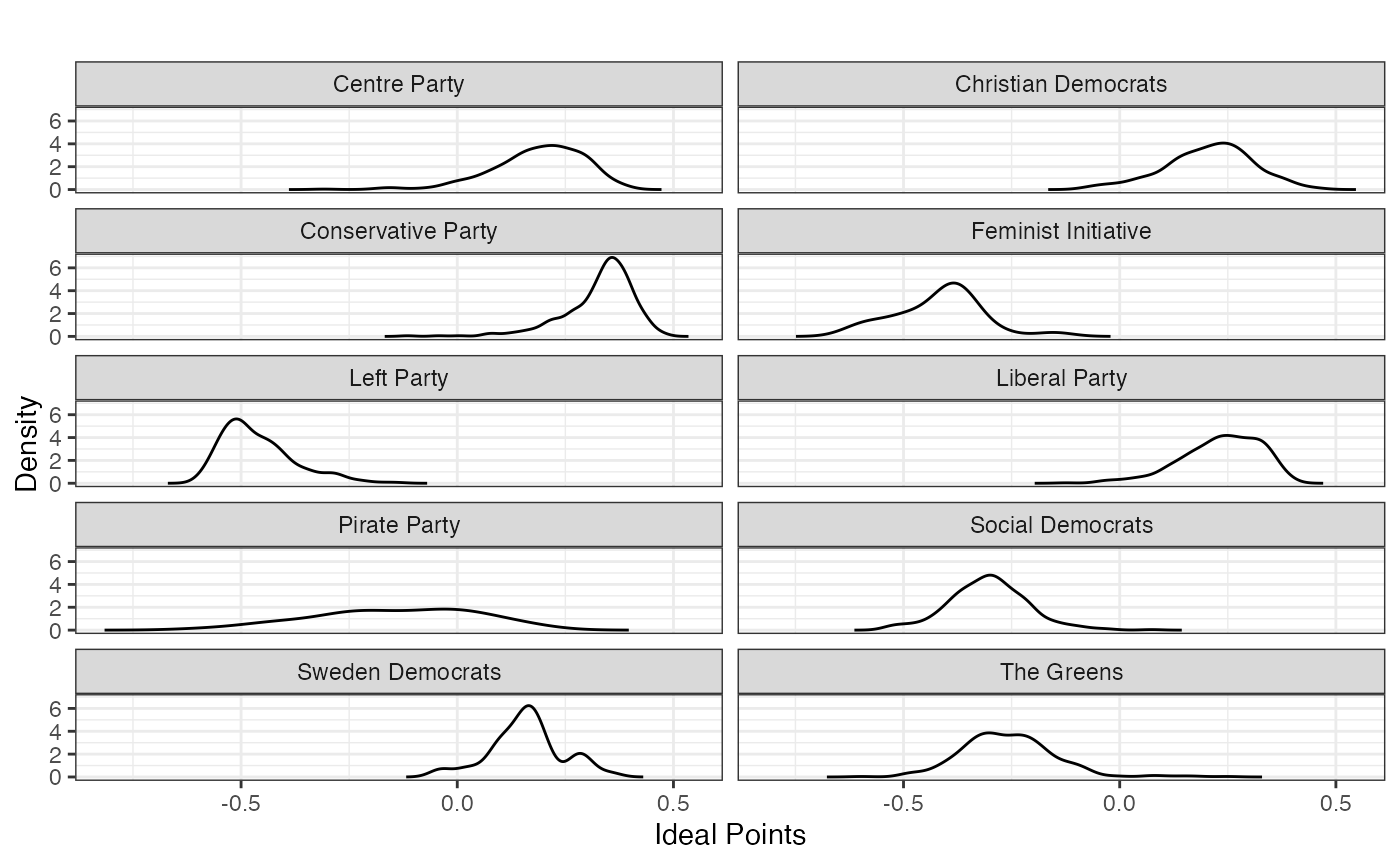
FIGURE 2.11: Basic Space (Blackbox) Scaling of 2010 Swedish Parliamentary Candidate Data (Candidates by Party)
Density plot syntax and comparison of defeated/elected candidates
# Keep only the parties of elected candidates, set others to NA
party.name.sweden[which(elected == 0)] <- NA
plot_resphist(result.sweden, groupVar=party.name.sweden, dim=1,  scaleDensity=FALSE) +
  facet_wrap(~stimulus, ncol=2) +
  theme(legend.position="none") +
  scale_color_manual(values=rep("black", 10))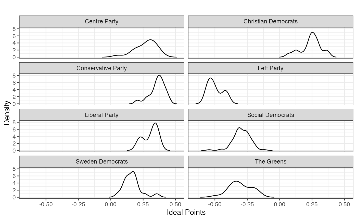
FIGURE 2.12: Basic Space (Blackbox) Scaling of 2010 Swedish Parliamentary Candidate Data (Elected and Defeated Candidates by Party)
2.2.3 Estimating Bootstrapped Standard Errors for Black Box Scaling
The 2010 Swedish parliamentary candidate data
# Candidate point estimates blackbox scaling
outbb <- boot.blackbox(issues.sweden, missing=8, dims=3, minscale=5,
                      verbose=FALSE, posStimulus=13)
Matrix creation for Swedish candidates
first.dim <- data.frame(
   point = result.sweden$individuals[[3]][,1],
   se = apply(outbb[,1,], 1, sd)
 )
first.dim$lower <- with(first.dim, point - 1.96*se)
first.dim$upper <- with(first.dim, point + 1.96*se)
first.dim$elected <- factor(elected, levels=c(0,1),
                            labels=c("Not Elected", "Elected"))
head(first.dim)
## point se lower upper elected
## 1 -0.355 0.10567674 -0.5621264 -0.14787359 Not Elected
## 2 -0.383 0.10634592 -0.5914380 -0.17456200 Elected
## 3 -0.335 0.09235433 -0.5160145 -0.15398551 Not Elected
## 4 -0.359 0.09925504 -0.5535399 -0.16446012 Not Elected
## 5 -0.206 0.09182988 -0.3859866 -0.02601343 Not Elected
## 6 -0.072 0.06757198 -0.2044411 0.06044109 Not ElectedPlot for the distribution of first dimensions bootstrapped SE
ggplot(first.dim, aes(x=se, group=elected)) +
  stat_density(geom="line", bw=.005) +
  facet_wrap(~elected) +
  theme(aspect.ratio=1) +
  xlab("Standard Error") +
  xlim(c(0,.2)) +
  theme_bw()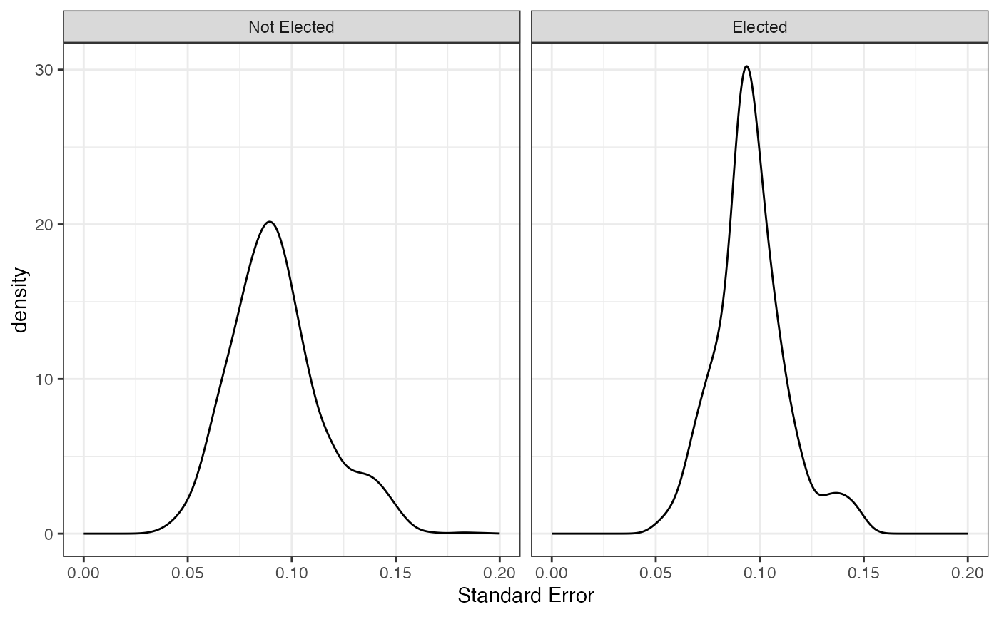
FIGURE 2.13: Basic Space (Blackbox) Scaling of 2010 Swedish Parliamentary Candidate Data with Boostrapped Standard Errors (Elected and Defeated Candidates)
To determine whether the difference between the two distributions is statistically significant, we compute a permutation test for the difference in standard errors variances.
# Variance test syntax
library(perm)
levels(first.dim$elected) <- c("No", "Yes")
permTS(se ~ elected, data=first.dim,
      alternative="greater", method="exact.mc",
      control=permControl(nmc=10^4-1))
##
## Exact Permutation Test Estimated by Monte Carlo
##
## data: se by elected
## p-value = 0.96
## alternative hypothesis: true mean elected=No - mean elected=Yes is greater than 0
## sample estimates:
## mean elected=No - mean elected=Yes
## -0.002516503
##
## p-value estimated from 9999 Monte Carlo replications
## 99 percent confidence interval on p-value:
## 0.9546745 0.96487402.3.1 Example 1: 2000 and 2006 Comparative Study of Elec- toral Systems (Mexican Modules)
##      PAN PRI PRD PT Greens PARM
## [1,]  11   6   1 99      6   99
## [2,]  11   6   5  5      5    5
## [3,]  10   4   3  3      8    3
## [4,]   8   9   7 99     99   99
## [5,]   9   5   3  4     99   99
## [6,]   9   6   1  1      9   99
Blackbox syntax for two datasets, with data cleaning arguments
library(basicspace)
result_2000 <- blackbox_transpose(mexicoCSES2000, missing=99,
                                  dims=3, minscale=5, verbose=TRUE)
result_2006 <- blackbox_transpose(mexicoCSES2006, missing=99,
                                  dims=3, minscale=5, verbose=TRUE)
Multiplying here to avoid negative scores
# Extract and transform dimensions for the year 2000
first.dim.2000 <- -1 * result_2000$stimuli[[2]][, 2]
second.dim.2000 <- result_2000$stimuli[[2]][, 3]

# Extract and transform dimensions for the year 2006
first.dim.2006 <- -1 * result_2006$stimuli[[2]][, 2]
second.dim.2006 <- result_2006$stimuli[[2]][, 3]

# Create a data frame for plotting
plot.df <- data.frame(
  dim1 = c(first.dim.2000, first.dim.2006),
  dim2 = c(second.dim.2000, second.dim.2006),
  year = rep(c(2000, 2006), c(length(first.dim.2000), length(first.dim.2006))),
  party = factor(c(rownames(result_2000$stimuli[[2]]), rownames(result_2006$stimuli[[2]])))
)

# Add nudge values for adjusting labels in the plot
plot.df$nudge_x <- c(0, 0, 0, 0, 0, -0.125, 0, 0, 0, 0.13, 0, 0, -0.225, 0)
plot.df$nudge_y <- c(-0.05, -0.05, 0.05, -0.05, -0.05, 0, -0.05, -0.05, -0.05, 0.03, 0.05, -0.05, -0.025, 0.05)

# Display the first few rows of the data frame
head(plot.df)
## dim1 dim2 year party nudge_x nudge_y
## 1 0.811 -0.292 2000 PAN 0.000 -0.05
## 2 0.120 0.903 2000 PRI 0.000 -0.05
## 3 -0.268 -0.100 2000 PRD 0.000 0.05
## 4 -0.338 -0.181 2000 PT 0.000 -0.05
## 5 0.048 -0.195 2000 Greens 0.000 -0.05
## 6 -0.373 -0.134 2000 PARM -0.125 0.00
ggplot(plot.df, aes(x=dim1, y=dim2, group=year)) +
  geom_point() +
  geom_text(aes(label=party), nudge_y=plot.df$nudge_y, size=3,
           nudge_x=plot.df$nudge_x, group=plot.df$year) +
  facet_wrap(~year) +
  xlim(-.55,1) +
  ylim(-.55,1) +
  theme_bw() +
  labs(x="First Dimension", y="Second Dimension")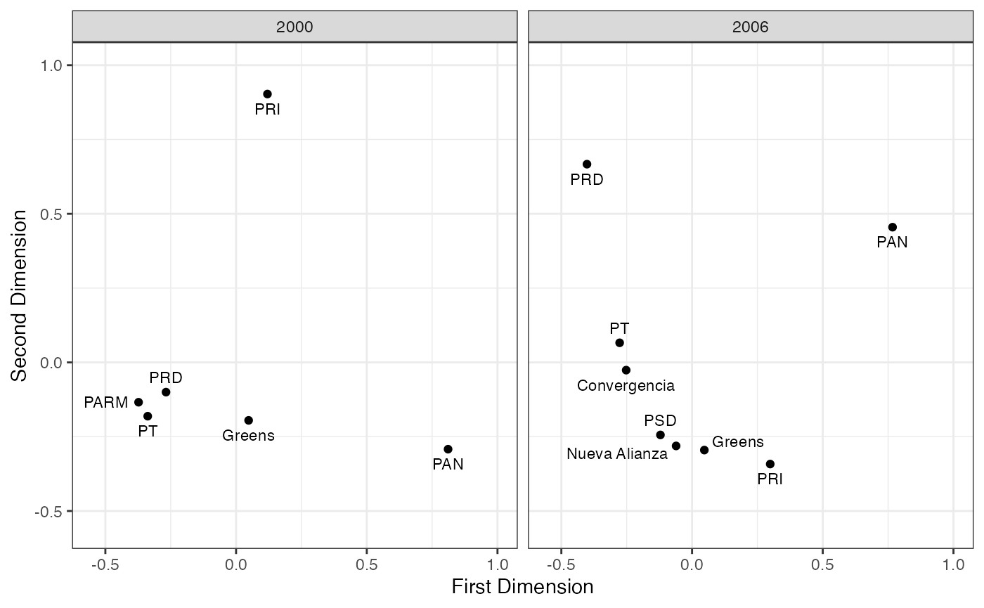
FIGURE 2.14: Basic Space (Blackbox Transpose) Scaling of Left- Right Placements of Mexican Political Parties (2000 and 2006 Com- parative Study of Electoral Systems)
2.3.2 Estimating Bootstrapped Standard Errors for Black Box Transpose Scaling
rankings <- as.matrix(franceEES2009[,2:9])
mode(rankings) <- "numeric"
original <- blackbox_transpose(rankings,
                     missing=c(77,88,89), dims=3, minscale=5, verbose=FALSE)
# Reverse check for the first stimulus
if (original$stimuli[[1]][1,2] > 0) {
    original$stimuli[[1]][,2] <- -1 * original$stimuli[[1]][,2]
}

# Print the fits from the original object
print(original$fits)
## SSE SSE.explained percent SE singular
## Dimension 1 15662.524 57751.39 78.665454 1.751592 241.07084
## Dimension 2 10224.214 63189.70 7.407739 1.562470 86.24658
## Dimension 3 7177.296 66236.61 4.150327 1.481290 62.02679
outbbt <- boot.blackbox_transpose(rankings, missing=c(77,88,89),
                                  dims=3, minscale=5, verbose=FALSE, R=5)
# Create a data frame for the bootstrapped results
france.boot.bbt <- data.frame(
  party = colnames(rankings),
  point = original$stimuli[[1]][, 2],
  se = apply(outbbt[, 1, ], 1, sd, na.rm = TRUE)
)

# Calculate the confidence intervals
france.boot.bbt$lower <- with(france.boot.bbt, point - 1.96 * se)
france.boot.bbt$upper <- with(france.boot.bbt, point + 1.96 * se)

# Display the resulting data frame
france.boot.bbt
## party point se lower upper
## 1 Extreme Left -0.453 0.03615660 -0.52386694 -0.38213306
## 2 Communist -0.327 0.01961632 -0.36544799 -0.28855201
## 3 Socialist -0.089 0.01190378 -0.11233141 -0.06566859
## 4 Greens -0.025 0.04033981 -0.10406602 0.05406602
## 5 UDF (Bayrou) 0.115 0.02334952 0.06923494 0.16076506
## 6 UMP (Sarkozy) 0.456 0.07369735 0.31155319 0.60044681
## 7 National Front 0.612 0.07037258 0.47406974 0.74993026
## 8 Left Party -0.290 0.01281796 -0.31512319 -0.264876812.4 Ordered Optimal Classification
##   libcon diplomacy iraqwar govtspend defense bushtaxcuts healthinsurance
## 1      4        NA      NA         3       7          NA               7
## 2      4         4       4         6       5           1               2
## 3      6         1       1         3       5           1               4
## 4      4         7       3         7       2           3               1
## 5      6         5       1         3       5           1               5
## 6      6         1       4         6       6           4               2
##   govtjobs aidblacks govtfundsabortion partialbirthabortion environmentjobs
## 1        7         7                 1                   NA               2
## 2        3         6                 4                    1               3
## 3        4         5                 4                    1               4
## 4        1         1                 3                   NA              NA
## 5        6         6                 4                    1               4
## 6        5         7                 4                    1              NA
##   deathpenalty gunregulations
## 1            1              1
## 2            4              1
## 3            2              1
## 4            4              3
## 5            2              3
## 6            4              3
The command below performs OOC on the 2004 ANES issue scale data in two dimensions:
issue.result <- ooc.result$issues.unique

# Set the row names of issue.result using the column names from issuescales
rownames(issue.result) <- colnames(issuescales)

# Print selected columns from issue.result
print(issue.result[, c("normVectorAngle2D", "wrongScale",
                       "correctScale", "errorsNull", "PREScale")])
## normVectorAngle2D wrongScale correctScale errorsNull
## libcon 5.308387 365 555 623
## diplomacy -14.617062 505 536 774
## iraqwar -1.432234 334 855 596
## govtspend 37.532690 501 559 776
## defense -3.807150 528 533 761
## bushtaxcuts -19.485846 219 560 456
## healthinsurance 46.666181 371 741 892
## govtjobs 42.263435 348 755 878
## aidblacks 36.393860 457 616 798
## govtfundsabortion -20.912765 472 669 603
## partialbirthabortion -32.859434 286 839 503
## environmentjobs -15.768729 529 490 744
## deathpenalty -18.939594 546 617 599
## gunregulations -7.835209 518 683 669
## PREScale
## libcon 0.4141252
## diplomacy 0.3475452
## iraqwar 0.4395973
## govtspend 0.3543814
## defense 0.3061761
## bushtaxcuts 0.5197368
## healthinsurance 0.5840807
## govtjobs 0.6036446
## aidblacks 0.4273183
## govtfundsabortion 0.2172471
## partialbirthabortion 0.4314115
## environmentjobs 0.2889785
## deathpenalty 0.0884808
## gunregulations 0.22571002.5 Using Anchoring Vignettes
calculate party means and standard deviations across all CHES experts
# Load the asmcjr package
library(asmcjr)

# Load the ches_eu dataset
data(ches_eu)

# Calculate the column means of sub.europe, ignoring NA values
means <- colMeans(sub.europe, na.rm = TRUE)

# Calculate the standard deviations of the columns in sub.europe, ignoring NA values
sds2 <- apply(sub.europe, 2, sd, na.rm = TRUE)

# Convert sub.europe to a matrix
sub.europe <- as.matrix(sub.europe)

# Ensure the mode of sub.europe is numeric
mode(sub.europe) <- "numeric"
Call the blackbox_transpose
library(basicspace)
result <- blackbox_transpose(sub.europe,dims=3,
                             minscale=5,verbose=TRUE)
##
##
## Beginning Blackbox Transpose Scaling...118 stimuli have been provided.
##
## Blackbox-Transpose estimation completed successfully.
# Create a data frame europe.dat containing x, y coordinates, means, party names, and types
europe.dat <- data.frame(
  x = -result$stimuli[[2]][,2],  # Negate the second column of stimuli and assign to x
  y = result$stimuli[[2]][,3],   # Use the third column of stimuli for y
  means = means,                 # Add the means calculated earlier
  party = colnames(sub.europe),  # Use the column names of sub.europe as party names
  type = car:::recode(means,     # Recode means into categories: Left, Moderate, and Right
    "lo:3 = 'Left'; 3:7 = 'Moderate'; 7:hi = 'Right'",
    as.factor = TRUE)
)

# Separate europe.dat into two data frames: parties.dat and vignette.dat
parties.dat <- europe.dat[-(1:3), ]  # Exclude the first three rows for parties.dat
vignette.dat <- europe.dat[(1:3), ]  # Include only the first three rows for vignette.dat

# Extract fit values from the result object
onedim <- result$fits[1, 3]  # Extract the one-dimensional fit value
twodim <- result$fits[2, 3]  # Extract the two-dimensional fit value
library(ggplot2)
ggplot(parties.dat, aes(x = x, y = y)) +
  geom_point(aes(shape = type, color = type), size = 3) +

  scale_color_manual(values = gray.palette(3)) +
  theme_bw() +
  # Add text labels "A", "B", and "C" to the points in vignette.dat
  geom_text(data = vignette.dat, label = c("A", "B", "C"),
            show.legend = FALSE, size = 10, color = "black") +
  xlab(paste0("First Dimension (fit = ", round(onedim, 1), "%)")) +
  ylab(paste0("Second Dimension (fit = ", round(twodim, 1), "%)")) +
  theme(legend.position = "bottom", aspect.ratio = 1) +
  labs(colour = "Party Group", shape = "Party Group")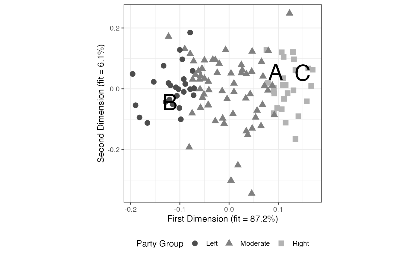
FIGURE 2.16: Result of Blackbox Transpose with Anchoring Vignettes
ggplot(parties.dat, aes(x=x, y=means)) +
  geom_smooth(method="loess", color="black", lwd=.5, se=FALSE) +
  geom_point(aes(shape=type, color=type), size=3) +
  scale_color_manual(values=gray.palette(3)) +
  theme_bw() +
  xlab("First Dimension Coordinates") +
  ylab("Mean Party Placement") +
  theme(legend.position="bottom", aspect.ratio=1) +
  labs(shape="Party Group", colour="Party Group")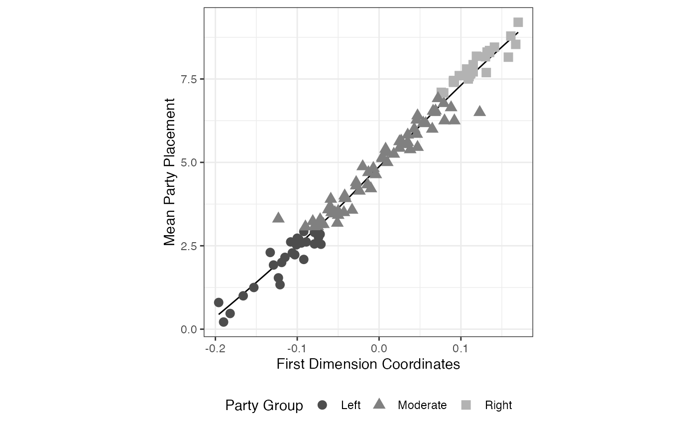
FIGURE 2.17: Result of Blackbox Transpose versus Mean Placementes